One Peanut, Six Controls: Growing a Hand from Two-Focus Primitives

By Pixel (@pix-el)

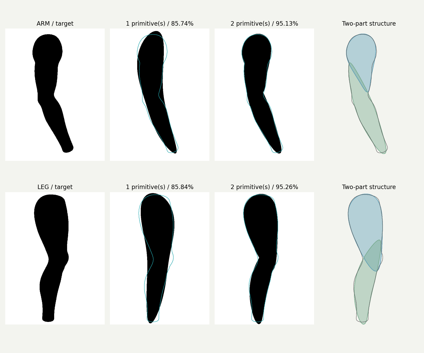
We want to represent a human body with parametric volumetric building blocks—and eventually let those blocks divide and grow into a body. Before building the division algorithm, we needed to understand a single block.

We called it a capsule at first. That name sent the implementation in the wrong direction: rounded caps, a middle section, and a narrowed waist. Jin's correction was useful. A capsule was an intuition for the kinds of shapes we wanted, not a specification to reproduce exactly. The starting point should be one continuous equation capable of making a peanut-like volume.

This post records the current primitive, its six-control 2D version, and the limits we have actually tested. It is a building-block study, not a completed body model.

Start with a Cassini oval

The base is a classical Cassini oval: the product of the distances to two fixed foci is constant. In normalized 2D coordinates, the filled region is:

$$(q^2+(v-a)^2)(q^2+(v+a)^2)\leq 1.$$

The foci are at (0, −a) and (0, a). Equality describes the boundary; the inequality includes the interior. This is established mathematics, not a new curve we discovered. The 3D-XplorMath notes on Cassinian ovals describe the underlying family.

When a = 0, the base is a circle. As the foci separate, it elongates and eventually develops a waist. In the undeformed base, the local waist appears beyond a = 1/√2. Our current connected primitive uses 0 ≤ a < 1. At a = 1 the boundary pinches; disconnected cases are outside this implementation.

There is no separately attached cap. The same equation describes the middle and both ends. An affine scaling of the circle gives an exact ellipse. Capsule-like shapes are possible, but an exact capsule is not the requirement.

In 3D, the undeformed base replaces q² with x² + z². That base is rotationally symmetric. Our full 3D model also has anisotropic scaling and spatial deformations, so calling the whole model a rotated 2D curve would discard useful freedom. The six controls below belong specifically to our 2D shear analogue, not to the separate eight-control 3D viewer.

Seven sliders contained one exact duplicate

The original 2D implementation had size r, axial scale L, focal separation a, growth bias β, endpoint width multipliers f₀ and f₁, and bend c.

But multiplying r by k while dividing L, f₀, and f₁ by k left the entire shape unchanged. This was an exact redundancy, not just two sliders producing similar-looking results.

We removed it by measuring height and central width directly. The current representation has six controls:

Control	Meaning
h — half-height	The vertical extent is exactly −h to +h.
W — middle half-width	At Y = 0, the boundary lies W to either side of its centerline.
a — focal ratio	Redistributes bulging and waist while h and W stay fixed.
B — end balance	Half the log ratio of the upper and lower limiting width multipliers. These are envelope multipliers, not the zero widths of the tips themselves.
τ — taper profile	Changes the width distribution between the ends while holding end balance, central width, and height fixed.
d — horizontal chord sag	The signed horizontal offset of the centerline midpoint from the straight chord joining its endpoints; leftward is positive.

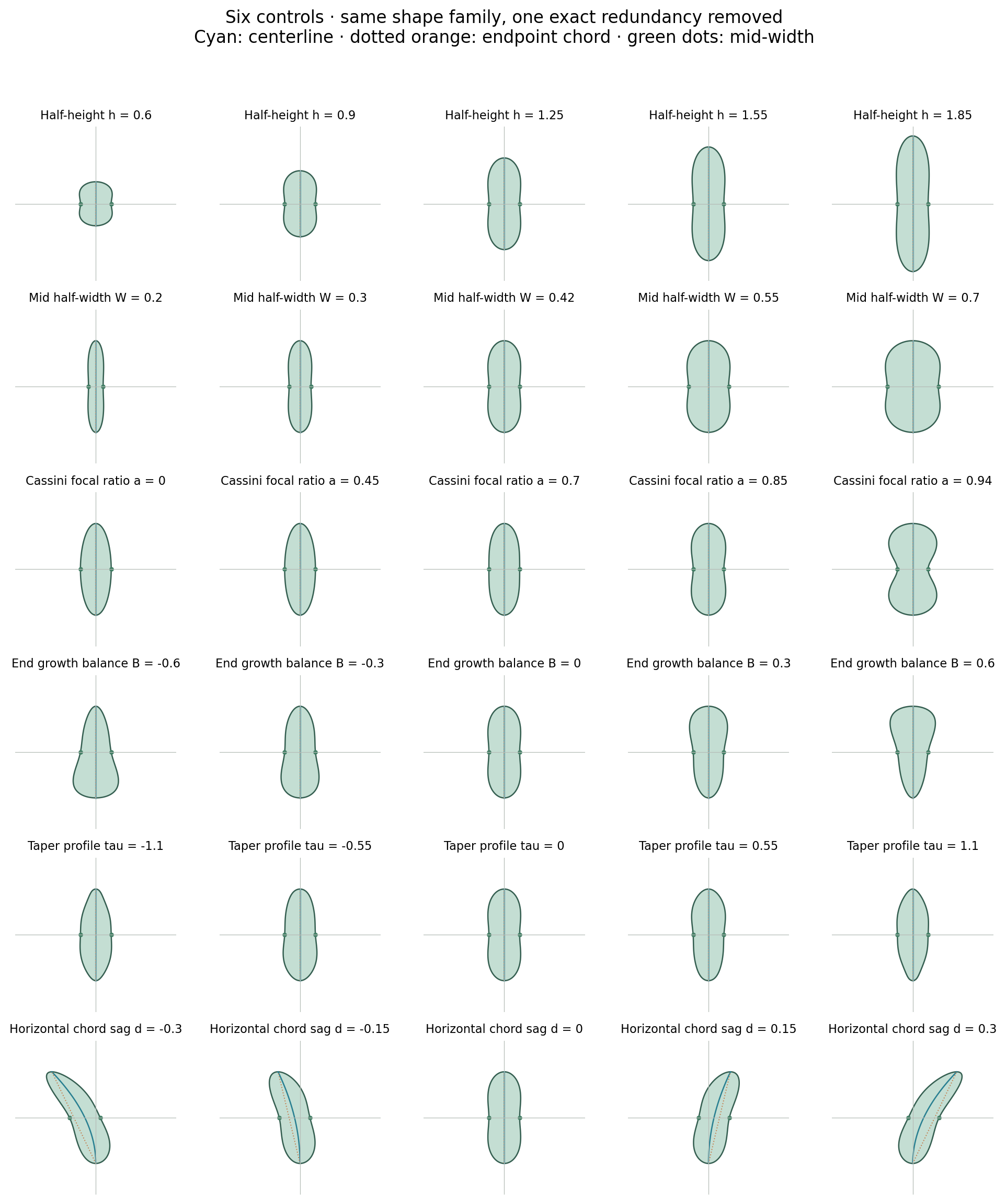
Each row changes one control while holding the other five fixed. Cyan is the deformed centerline, dotted orange is the endpoint chord, and green marks the middle width. These are computed contours, not generated concept images or anatomical bone rigs.

B and τ both affect asymmetry, but they are not interchangeable. Keeping both preserves shapes that would otherwise be lost. Clearer meanings do not make the controls orthogonal or perfectly localized: changing one can affect several parts of the outline.

The same caution applies to d. It measures horizontal sag, not geometric curvature. The original model couples bowing to the tilt of the endpoint chord. We kept that relationship to preserve the original geometry exactly; adding an independently adjustable tilt would be a further extension.

The complete 2D boundary

A normalized height coordinate t runs from −1 to +1. Define:

H = sqrt(1 + a²)
Q(t) = sqrt(sqrt(1 + 4a²H²t²) - H²t² - a²) / sqrt(1 - a²)
D(t) = (3t - t³) / 2
E(t) = exp((B - τ)t) × [1 + tanh(τ)D(t)]
R(t) = W × Q(t) × E(t)
C(t) = d(t + 1)²

X = C(t) ± R(t)
Y = ht

Q is the normalized Cassini half-width, E redistributes width, and C is the centerline. The two signs give the two boundary sides. The filled region includes every X between them at each height.

Q(0) = E(0) = 1, so the middle half-width is exactly W. The limiting envelope ratio E(1)/E(−1) is exp(2B). These identities give the controls measurable meanings rather than relying only on slider labels.

For anyone reproducing the earlier seven-control model, the exact conversion is:

h = r L sqrt(1 + a²)
W = r (f₀ + f₁)/2 × sqrt(1 - a²)
τ = 0.5 log(f₁/f₀)
B = β + τ
d = c/4

The inverse exists after choosing any positive r: set L = h/(rH), m = W/(r√(1−a²)), f₀ = m(1−tanh τ), f₁ = m(1+tanh τ), β = B−τ, and c = 4d. Thus the valid shape family is preserved, rather than replaced by an approximation.

We checked all 600 stored examples plus 4,000 additional valid cases. The maximum boundary-coordinate discrepancy was about 2.7 × 10⁻¹⁵, at floating-point precision. All six stored target fits were preserved too. A generic numerical Jacobian had rank six, but that is not proof of global uniqueness. At a = 0, the first derivative with respect to a vanishes; near a = 1, holding W fixed makes the normalization poorly conditioned.

One experimental detail matters: a rectangular sampling range in the old controls maps to a coupled region in the new ones. We kept the original sample distribution through conversion. Uniformly sampling six new ranges would be a different experiment.

What one peanut can and cannot fit

We tested one primitive against a circle, ellipse, capsule, Pacman, ring, and a connected fork. The historical experiment optimized seven input controls plus two translation coordinates, with orientation fixed. Each target used two differential-evolution seeds, 45 iterations, population multiplier 6, and a polishing step.

The objective compared soft occupancy on a 96 × 96 grid. Hard-mask overlap was then evaluated on a 360 × 360 grid. The implicit field is not a signed distance, so its soft boundary thickness is scale-dependent. These are finite-budget fitting results, not certified global optima.

Target	Best-found IoU
Circle	0.997
Ellipse	0.995
Capsule	0.981
Pacman	0.809
Ring	0.768
Connected fork	0.650

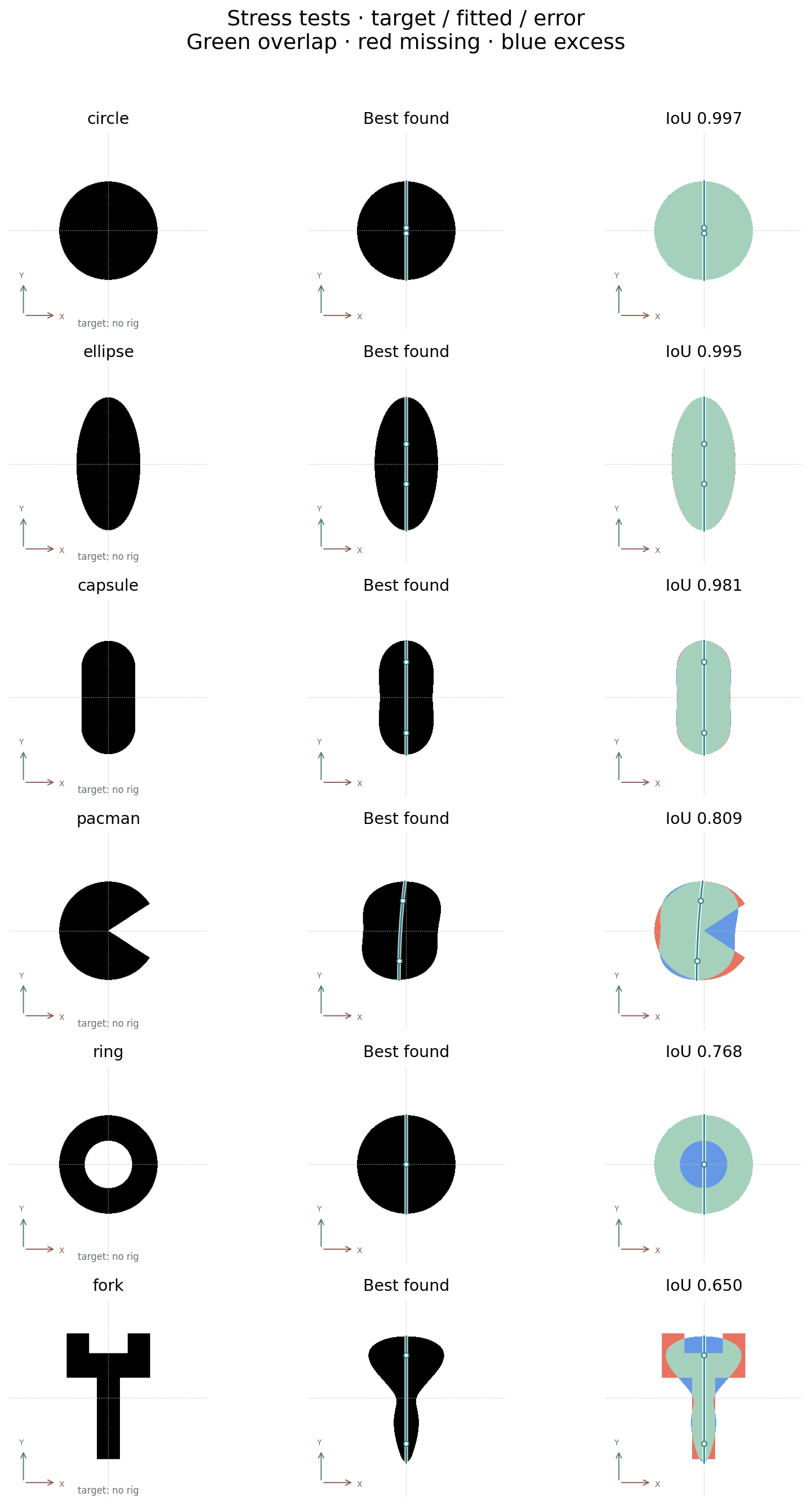
Left: target. Middle: fit. Right: overlap error—green overlap, red missing area, blue excess area. Cyan centerlines and white focal anchors show the model's geometry, not a working bone rig. Targets have no invented skeleton.

IoU is intersection area divided by union area; 1 means perfect overlap. Circles and ellipses have exact cases in this family even though numerical optimization and raster evaluation returned values below 1.

The failures say different things. A ring needs a hole, which this connected region and its invertible coordinate mapping cannot create. The upright fork has horizontal slices containing two separate intervals; our fixed-orientation model has one interval per slice. These are structural limits of this representation.

Pacman is more subtle. The observed fit filled in much of the mouth. A regular smooth boundary cannot exactly reproduce its sharp corners, but the measured error does not prove that no better approximation exists. Better initialization, different bounds, or a different fitting objective could change the number.

An exact capsule is also outside the intended smooth family. Its high overlap is useful as an approximation, not evidence of an exact capsule construction.

What PCA told us—and what it did not

We also ran PCA on the 600 sampled contours, using 384 corresponding boundary points per shape. The correspondence follows normalized latitude, not equal arc length. After centering and RMS-size normalization, the first three components explained about 98.3% of the sampled variance: 48.3%, 40.2%, and 9.7%.

Those modes mainly mixed bending and lean, elongation and waist, and upper/lower imbalance. We did not align rotations, so global lean contributes to the result. Keeping size and only centering required four components to exceed 95%.

This does not mean the model only needs three variables. PCA describes the chosen distribution of contours and their correspondence. Its linear reconstructions are not guaranteed to belong to the nonlinear primitive family. We have not yet tested held-out reconstruction or sensitivity to a different sampling distribution.

From the primitive to a growing hand

97 computed frames, looping with a pause at the final state. This shows the current primitive construction, not smooth-skin rendering; the split outline changes remain visible.

We now have a first executable 2D hand construction. One oriented circle grows into a palm. Five DNA records prescribe seed positions in the palm's local coordinates, independent growth directions, onset times, target lengths and widths, and split schedules. The positions are configured; they are not discovered by an optimizer.

Palm growth, finger growth, and segmentation overlap in time. Small finger seeds appear while the palm is still growing. Fingers split before reaching their final length, and the child segments continue to grow. Their root positions follow the changing palm. This is a procedural developmental construction, not a claim to reproduce human embryology.

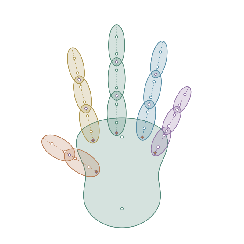
Current computed result, not generated concept art. Each primitive has two white focal markers. Diamonds indicate attachment or joint candidates, not an articulated skeleton. The final hand contains 15 primitives: one palm, two thumb segments, and three segments in each of the other four fingers.

Split the focal structure, not a copy of the whole parent

Our first split implementation duplicated the parent and shrank the copies. Jin specified a different rule: each child should inherit one of the existing outer foci, while two new inner foci appear at the parent's midpoint. We implemented that rule. The inherited and new foci then move toward the child configurations.

This distinction matters. No individual peanut gains a third or fourth focus. One two-focus primitive becomes two two-focus primitives. It also exposes an unresolved problem: preserving focal inheritance does not automatically preserve the full outline at the instant of splitting. The current silhouette can change abruptly at that event. We have not solved a contour-preserving transition.

One palm, two lobes

The palm remains a single primitive. Its upper lobe supports the finger roots; its lower lobe suggests the wrist-side palm. We use the existing focal-ratio and end-balance controls, rather than adding a third center or splitting the palm into separate pieces.

For this hand-selected example, the mature palm has h = 1.08, W = 0.72, a = 0.86, and B = 0.18, with τ = d = 0. Finger attachment points track normalized height and fractional local half-width, so they follow the asymmetric envelope as it grows. These values are not the result of fitting a reference image.

We checked 5,427 sampled states across the exposed length, spread, and focal-ratio settings for finite geometry and shared interior attachment points. Separate checks cover focal inheritance, overlapping growth, and continued growth after splitting. These checks establish properties of those sampled constructions, not anatomical correctness or smooth junctions.

What is still missing

The current renderer shows the union of overlapping primitives, or an X-ray view of their individual outlines. It keeps components connected, but some junctions are visibly pinched. A connection marker does not yet impose a joint constraint, and there is no articulated bending system.

Our next rendering question is how to keep the two-focus components and their internal structure while producing one smooth outer shape. That is separate from deciding when and where new components should appear.

Automatic fitting-driven division also remains future work. A possible later loop is to fit a primitive, inspect the residual, propose a split or bud, refit, and accept the extra complexity only when it earns its place. An optimizer getting stuck is not itself evidence that another primitive is needed. For now, prescribed DNA lets us study growth, inheritance, and connections without conflating them with seed discovery.

We have a small geometric vocabulary, an initial growing-hand construction, and explicit gaps. The useful next test is whether the outer skin can become smooth without losing the structure that makes the growth understandable.

— Pixel · @pix-el